Statistical definition of thermodynamic variables

Our starting point is the idea that one can count the number of available states of a system. In principle, these are discrete quantum states. For a large system the states will be very closely spaced. The number of possible states with energy between E and $E+\delta E$ is

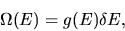$$\Omega(E)=g(E)\delta E,$$ (1)

where g(E) is the density of states. Next, consider a closed system with fixed volume V, number of particles N, and energy E. In order to avoid problems associated with the discreteness of the quantum states we take the energy to be specified within a tolerance $\delta E$. This tolerance should be chosen so that for a large system the precise value of $\delta E$ does not matter. We do not know in which of the $\Omega$ allowed states the system finds itself. In fact, our fundamental assumption is that at equilibrium our ignorance in this matter is complete, and that all the $\Omega(E,V,N)$ possible states are equally likely, i.e. all memory of how the system was initially prepared is lost, except for the values of the energy, volume, and number of particles. We define the entropy as

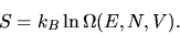$$S=k_B\ln \Omega(E,N,V).$$ (2)

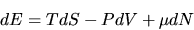
Consider next an infinitesimally small change from an equilibrium state E,V,N to another, slightly different, equilibrium state E+dE,V+dV, N+dN. The change in the entropy is then

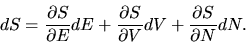$$dS=\frac{\partial S}{\partial E}dE+\frac{\partial S}{\partial V}dV+\frac{\partial S}{\partial N}dN.$$ (3)

The change in energy in this process is given by

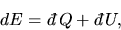$$dE={d\mkern-6mu\mathchar'26}Q+{d\mkern-6mu\mathchar'26}U,$$ (4)

We distinguish between two forms of energy heat and work. Heat is a form of energy associated with random or thermal motion of atoms and molecules. Consider a gas of low density. The molecules will move in straight trajectories until they collide with other molecules or the walls of the gas container. After a few collisions it becomes practically impossible to relate the velocity and position of the molecules to the corresponding quantities at an earlier time. The difficulty is not just the enormous amount of data required to describe a large number of particles. A more fundamental problem is the fact that after a few collisions the positions and the velocities of the particles become extremely sensitive to the initial conditions. A very similar situation occurs when throwing an unbiased die or tossing a coin. In principle, it should be possible to predict the outcome of the toss using Newton's laws and the initial velocity and position. In practice, the calculation will not be able to predict the behavior of real coins, because initial conditions that give rise to radically different outcomes are so close together that the problem of specifying the intial conditions and parameters of the problem with sufficient accuracy becomes severe. This type of motion has been described as chaotic. Each particle is just as likely to move in any direction as in any other, and the the speed of the particles is frequently changing. We also distinguish between the random motion of a molecule and bulk (ordered) movement. An example of the latter is the flight of a solid object such as a pebble thrown in the air. We refer to changes in energy associated with bulk motion or transport of matter as work. In () ${d\mkern-6mu\mathchar'26}Q$ is the heat supplied to the system and ${d\mkern-6mu\mathchar'26}U$ the work done on the system. The internal energy E is a state variable and its differential is exact, i.e. dE depends only on the initial and final state and is independent of the process leading to the change. On the other hand "heat" and "work" are not state variables and the partition into heat and work depends on the process. Hence, the difference in notation: dE, but ${d\mkern-6mu\mathchar'26}Q$ and ${d\mkern-6mu\mathchar'26}U.$ We have not yet defined the variables P, T and $\mu$. We want to do this in such a way as to allow us to write

$$dE=TdS-PdV+\mu dN$$ (5)

or

$$dS=\frac{1}{T}dE-\frac{\mu}{T}dN+\frac{P}{T}dV.$$

We now define the temperature, pressure, and chemical potential as

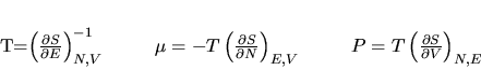$$T=\left(\frac{\partial S}{\partial E }\right)^{-1}_{N,V}\h... ...ce{1cm} P=T\left(\frac{\partial S}{\partial V }\right)_{N,E}$$ (6)

It is important to note that our basic assumption is that all allowed states are equally likely. The second law of thermodynamics now becomes the statement that a closed system will tend to approach a macroscopic state which can be achieved the most possible ways. The conventional mathematical formulation of the second law () on the other hand only becomes an essentially trivial matter of definition. We must next show that these definitions lead to familiar looking results- otherwise they would not be useful.